Table of Contents
Turbulent Diffusion
Author: Sarah Aepli
Rewritten by: Franziska Genter, Magdalena Gisiger, Judith Riedo
Turbulent Flow and Turbulent Diffusion
Turbulence is a term, which is known and used in daily life, mostly regarding aviation and weather forecasts.
There is no exact definition of a turbulent flow, but it is characterized by its irregularity, diffusivity, large Reynold Number, three-dimensionality, dissipation and continuum. To keep up its turbulence, the flow needs to be constantly receiving energy. The system is doing this by transferring energy from the small scale eddies to the larger ones in a cascade process. [1]
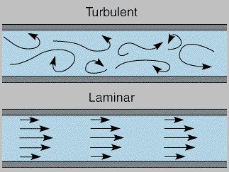
From the outside, there is no pattern of movement to be detected in a turbulent flow, the motions in the body are chaotic. Due to that fact, the diffusivity in the system increases. This results in the facilitated transport of mass, monumentum and heat throughout all layers. [1]
Figure comparing a laminar and a turbulent flow [2]
Reynolds number
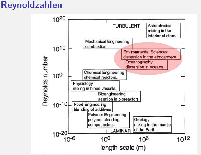
Reyonlds number is a dimensionless quantity that is used to help predict similar flow patterns in different fluid flow situations. The concept was introduced by George Gabriel Stokes in 1851 and named after Osborne Reynolds, who popularized its use in 1883.[3] Reynolds Number compares the non-linear, advective term with the damping, viscous term in the momentum equation. [9]
If the fluid medium is assumed to be incompressible \begin{equation*} \vec{\bigtriangledown} \vec{u} = 0 \end{equation*} and of uniform density, the entire dynamical configuration is specified by the strength of the incident stream $U$, the kinematic viscosity $v$ and the diameter of the cylinder (length) $L$. [4]
These external parameters combine to form one dimensionless number: [9]
\begin{equation*} $ \mathsf{Re} $ = \frac{UL}{\ v} \end{equation*}
The Reynolds number indicates if a flow is turbulent or laminar. For each system there is a critical Reynolds number $ \mathsf{Re_c_r_i_t} $ beyond which the flow is turbulent.
Reynolds Averaging
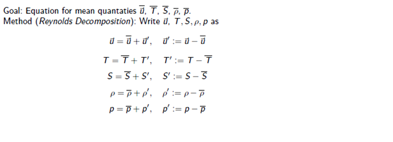
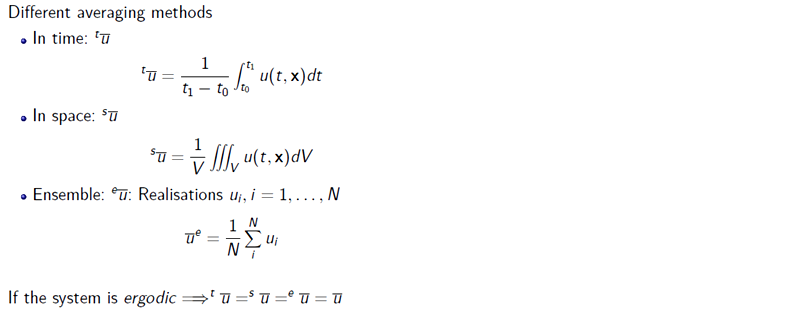
In a turbulent fluid, a field variable measured at a point generally fluctuates rapidly in time as eddies of various scales pass the point. In order that measurements be truly representative of the large-scale flow, it is necessary to average the flow over an interval of time long enough to average out small-scale eddy fluctuations, but still short enough to preserve the trends in the large-scale flow field. To do this we assume that the field variables can be separated into slowly varying mean fields and rapidly varying turbulent components. Following the scheme introduced by Reynolds, we then assume that for any field variables, the corresponding means are indicated by overbars and the fluctuating components by primes. [5][9]
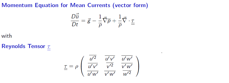
Reynolds Tensor τ describes the influence of the turbulence on the mean flow. The form and strength of Reynolds stress tensor depends on the turbulent flow and not on the fluid. [9]
Turbulence closure problem
When analyzing circulating systems we have six fundamental equations, like conservation of mass, momentum, heat and water vapor, and six unknown variables. This system is called closed because all the equations can be solved [6]. But when computing turbulent flows there is a fundamental difficulty due to the fact that, next to the fundamental unknowns $v$, $p$ and $T$, these equations also contains the Reynold stresses, the components of correlation and the turbulence dissipation. This leads to fewer fundamental equations than unknowns. In order to calculate the turbulence flow, this system has to be closed. This problem is called the turbulence closure problem [7].
Solutions can be found by providing additional model equations or making assumption [8].
The simplest closure is the k-theory, which assumes that the Reynolds stress behaves like molecular stress and they therefore balance each other out [7].
This model consists of two additional equations:
- 1st order turbulent closure
\begin{equation*} \tau = k \vec{\bigtriangledown} \vec{u} \end{equation*}
- Momentum equation for the mean flow
\begin{equation*} \frac{D\vec{u}}{\ Dt}} = \vec{g} - \frac{1}{\ \rho}} \vec{\bigtriangledown} p + \frac{k}{\ \rho} \bigtriangledown^2 \vec{u} \end{equation*}
With these assumptions the momentum equation for the mean flow has exactly the same form as the equation for the momentum itself [9].
References
[1] Fluid mechanics, turbulent flow and turbulence modeling, Lars Davidson (2015), Division of Fluid Dynamics, Department of Applied Mechanics, Chalmers University of Technology, Göteborg, Sweden
[2] Figure Turbulent Flow http://www.expertsmind.com/CMSImages/2110_laminar%20and%20turbulent.png
[3] Reynolds Number, Wikipedia (2015), http://en.wikipedia.org/wiki/Reynolds_number, Access: 22.03.15
[4] Introduction to Environmental Fluid Dynamics, H. Wernli, S. Pfahl (2014), Institute for Atomospheric and Climate Science, ETH Zürich
[5] An Introduction to Dynamic Meteorology, James R. Holton (2004), 4th edition, Elsevier
[6] Modeling the Atmospheric Boundary Layer (2), Jialin Lin (2012), Department of Geography and Environmental Science Graduate Program (ESGP), The Ohio State University, Lecture slides, lightning.sbs.ohio-state.edu/geo622/ch5_model2.ppt, Access: 21.03.2015
[7] Boundary Layer Theory, Schlichting Herrmann, Gersten Klaus (2000), 8th revised and enlarged edition, Springer
[8] Turbulence modelling, Ron Zevenhoven (2012), Åbo Akademi University, Thermal and Flow Engineering Laboratory, Lecture slides, http://users.abo.fi/rzevenho/iCFD12-RZ4.pdf, Access: 21.03.2015
[9] Mixing II: Turbulent Transport, Dr. Matthias Münnich (2015), Introduction to Physical Oceanography, ETH Zurich, Lecture slides, https://moodle-app2.let.ethz.ch/pluginfile.php/12823/mod_resource/content/5/Vorlesungsfolien/physocean15L5_handout_final.pdf, Access: 21.03.2015
